PCAPs and PANDAS

In a previous post I reviewed how you can use EDA techniques to programmatically pull data from the Mist dashboard for large-scale analysis. But what if you don’t have access to the Mist dashboard – or if you need to work with a raw PCAP that has been provided?

Packets don’t lie but a picture is worth a thousand words:

In this case we will be debugging RADIUS traffic to and from authentication servers to see if we can determine trends, measure performance, and identify anomalies. You’ll need several things to follow along:

• Working Python/Jupyter environment with the necessary modules
• A PCAP of RADIUS traffic flowing between your network access devices and the authentication servers
• A list of the IP addresses used by your authentication servers

If you are a Mist customer you can easily grab the PCAP by triggering a site-wide streaming PCAP from the AP ethernet ports with filters applied to only snag RADIUS traffic. Otherwise you can probably grab it from the WAN edge or at the RADIUS server itself.

Start by importing the necessary modules and setting up nest_asyncio so that pyshark can work within Jupyter:

import pyshark
import pandas as pd
import nest_asyncio
import seaborn as sns
import matplotlib.pyplot as plt
nest_asyncio.apply()

Next, we’ll define two functions – one that converts the pcap into a dataframe with the relevant information and one that analyzes that dataframe.

This module scans through the provided pcap and looks for RADIUS traffic. If RADIUS traffic is found it snags relevant fields like source/destination information, radius code, calling station, and the time and adds the entries into a dataframe. It also drops accounting traffic.

def pcap_to_dataframe(input_pcap):
    cap = pyshark.FileCapture(input_pcap)
    data = []

    for packet in cap:
        if hasattr(packet, "ip"):
            if 'radius' in packet:
                radius_layer = packet.radius
                code = int(radius_layer.code)
                if code == 1:
                    code = 'Access-Request'
                if code == 11:
                    code = 'Access-Challenge'
                if code == 2:
                    code = 'Access-Accept'
                if code == 3:
                    code = 'Access-Reject'
                if hasattr(radius_layer, 'Calling_Station_Id'):
                    calling_station = radius_layer.Calling_Station_Id
                else:
                    calling_station = 'not presented'
                data.append({
                    "src_ip": packet.ip.src,
                    "dst_ip": packet.ip.dst,
                    "src_port": packet.udp.srcport,
                    "dst_port": packet.udp.dstport,
                    "protocol": packet.transport_layer,
                    "radius code": code,
                    "calling_station": calling_station,
                    "time": packet.sniff_time.timestamp()
            })

    df = pd.DataFrame(data)
    df = df.drop(df[df['radius code'] == 4].index)
    return df

The following module is a little more complicated. I am also not a formal programmer, so I’m sure that there are better ways to do this… but it works!

Here’s what this is accomplishing:

• First, it identifies the unique network access devices in the environment – the network hardware that is sending requests to the authentication servers.
• Next, it sifts through the larger dataframe and creates unique dataframes for each of those network device for analysis.
• From each unique device dataframe it looks for different UDP ports that were used in the conversations. These ports are used by the network hardware to keep track of the different authentication requests. We create yet another subset of dataframes for each conversation seen from the specific network device.
• From here, we iterate through the conversations using a “session tracker” to identify the start and the end of an authentication. When we see the first “Access-Request” we start tracking a session and we keep going until we find an “Access-Accept” with the same NAD IP and UDP port. Once the loop is closed for each authentication we grab the relevant details from the starting and ending frames and add them to a new table.
  • Few caveats here – this does mean that we will not track an authentication that does not successfully complete. This also means that we need to see both the beginning and the end of the attempt in the pcap.

def radius_latency(df, radius_servers):
    unique_df = df[~df['src_ip'].isin(radius_servers)]
    unique_aps = list(unique_df['src_ip'].unique())
    results = []
    for each in unique_aps:
        ap_df = df[(df['src_ip'] == each) | (df['dst_ip'] == each)]
        unique_request = list(ap_df['src_port'].unique())
        if '1812' in unique_request:
            unique_request.remove('1812')
        for entry in unique_request:
            request_df = ap_df[(ap_df['src_port'] == entry) | (ap_df['dst_port'] == entry)]
            request_df = request_df.sort_values(by='time')
            request_df = request_df.to_dict('records')
            session_tracker = 0
            for i in range(len(request_df)):
                if request_df[i]['radius code'] == 'Access-Request' and session_tracker == 0:
                    initiate_frame = request_df[i]
                    session_tracker = 1
                elif request_df[i]['radius code'] == 'Access-Accept' and session_tracker == 1:
                    end_frame = request_df[i]
                    session_tracker = 0
                    nad_ip = initiate_frame['src_ip']
                    port = initiate_frame['src_port']
                    radius_server = initiate_frame['dst_ip']
                    calling_station = initiate_frame['calling_station']
                    start_time = initiate_frame['time']
                    end_time = end_frame['time']
                    totaltime = end_time - start_time
                    entry = {"calling_station": calling_station, "supplicant" : nad_ip, "nad_ip": radius_server, "port": port, "total time": totaltime}
                    results.append(entry)
    dataframe = pd.DataFrame(results)
    return dataframe

In the end we will have a dataframe that has an entry for each full RADIUS auth with the calling station, NAD IP address, radius server IP address, port, and the total time for the authentication process.

radius_servers = [A, B, C, D]
pcapdf = pcap_to_dataframe("Your_PCAP.pcapng")
df = radius_latency(pcapdf, radius_servers)

Now we can start applying our data analysis toolbox:

df.describe()

This does a quick analysis of the numerical columns in your dataframe – in this case, the total time from the initial Access-Request to Access-Accept.

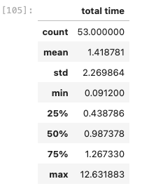
We can see here that we captured 53 full authentications and we saw some outliers. The mean was 1.412s, the median was 0.987s- but the max is 12.632s. To confirm the presence of outliers we can use a boxplot:

sns.boxplot(data=df, x='total time')

The boxplot, also known as a five-number summary plot, quickly shows the minimum value, first quartile, median, third quartile, and the maximum value. In this case it is showing us we have some very defined outliers in the data, shown as dots outside of the whiskers. Outliers in a boxplot are classified as follows:

• Minimum outliers – Q1(first quartile) – 1.5*IQR(interquartile range)
• Maximum outliers – Q3(third quartile) + 1.5*IQR(interquartile range)

You can break this out further to see which RADIUS servers are responsible for these outliers by modifying the boxplot:

sns.boxplot(data=df, x='radius_server', y='total time')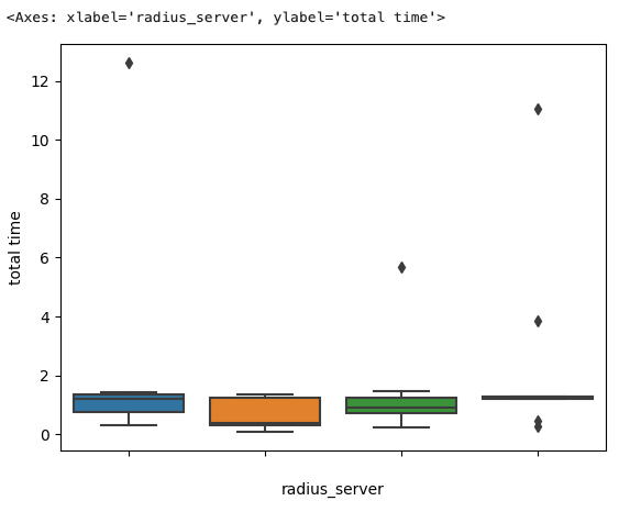

You can also get a feel for the shape of the data for each radius server by creating a histplot with the radius_server set to be the data hue:

plt.figure(figsize=(20,7))
sns.histplot(data=df, x='total time', hue='radius_server', bins = 48,kde=True)
plt.show()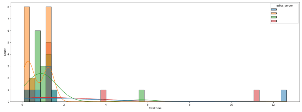

If you don’t want the data for each server to overlap you can also break out the histplot into multiple rows by using FacetGrid:

g = sns.FacetGrid(df, row='radius_server', sharey = False, aspect=4, palette='Set1')
g.tick_params(axis='x', labelbottom=True)
g.map(sns.histplot, "total time", kde=True)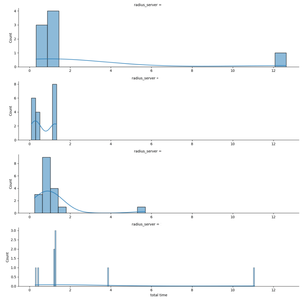

We can clearly see that two radius servers had lengthy authentication times that would impact the client. The ‘standard’ performance of each RADIUS server is fairly healthy though, so we want to see what happened to cause those outliers. To get the details on these records, do a quick sort_values function within the dataframe:

df.sort_values(by=['total time'], ascending=False).head(5)

This will give you the five longest authentications seen in the pcap along with the information on the calling station, the AP/switch, the RADIUS server, and the port that was used to negotiate. Now that you know what you are looking for it’s a simple matter to go back to the Wireshark capture and apply a filter so you can look deeper into the relevant packets:

ip.addr == {nad_ip} && udp.port == {port}

In this case it uncovered that there were clients experiencing intermittent lengthy authentication times due to a disagreement between the client and the RADIUS server on the session duration. The client would NAK the first attempt, resulting in a Access-Reject, and then try again with a full authentication.

Hopefully this entry shows how leveraging these techniques allows you to quickly assess the health of the network and determine where to go next.

As a footnote you will sometimes see outliers that don’t make sense to include when you use this code. This can happen if you have an extensive pcap running and the AP attempted to authenticate one client, never got a response to close out the session_tracker in the code, and then selected the same port to negotiate a connection for another client that was eventually accepted. If you run into this you can choose to drop the outliers from the dataframe by using:

df = df.drop(index=123)